Available with Image Server
The Calculate Density tool calculates the density of features in a neighborhood around those features. It can be calculated for both point and line features.
Possible uses include analyzing density of housing or occurrences of crime for community planning purposes or exploring how roads or utility lines influence wildlife habitat. The population field can be used to weight some features more heavily than others or allow one point to represent several observations. For example, one address may represent a condominium with six units, or some crimes may be weighted more heavily than others in determining overall crime levels. For line features, a divided highway may have more impact than a narrow dirt road.
How kernel density is calculated
Kernel density is calculated differently for different features.
Point features
Calculate Density calculates the density of point features around each output raster cell.
Conceptually, a smoothly curved surface is fitted over each point. The surface value is highest at the location of the point and diminishes with increasing distance from the point, reaching zero at the Search radius distance from the point. Only a circular neighborhood is possible. The volume under the surface equals the Population field value for the point, or 1 if NONE is specified. The density at each output raster cell is calculated by adding the values of all the kernel surfaces where they overlay the raster cell center. The kernel function is based on the quartic kernel function described in Silverman (1986, p. 76, equation 4.5).
If a population field setting other than NONE is used, each item's value determines the number of times to count the point. For example, a value of 3 will cause the point to be counted as three points. The values can be integer or floating point.
By default, a unit is selected based on the linear unit of the projection definition of the input point feature data or as otherwise specified in the Output Coordinate System environment setting.
If an output Area units factor is selected, the calculated density for the cell is multiplied by the appropriate factor before it is written to the output raster. For example, if the input units are meters, the output area units will default to Square kilometers. The end result of comparing a unit scale factor of meters to kilometers will result in the values being different by a multiplier of 1,000,000 (1,000 meters × 1,000 meters).
Line features
Kernel Density can also calculate the density of linear features in the neighborhood of each output raster cell.
Conceptually, a smoothly curved surface is fitted over each line. Its value is greatest on the line and diminishes as you move away from the line, reaching zero at the specified Search radius distance from the line. The surface is defined so the volume under the surface equals the product of line length and the Population field value. The density at each output raster cell is calculated by adding the values of all the kernel surfaces where they overlay the raster cell center. The use of the kernel function for lines is adapted from the quartic kernel function for point densities as described in Silverman (1986, p. 76, equation 4.5).

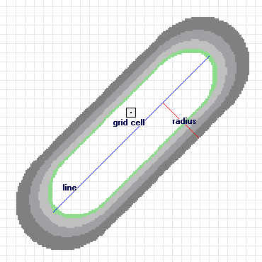
The illustration above shows a line segment and the kernel surface fitted over it. The contribution of the line segment to density is equal to the value of the kernel surface at the raster cell center.
By default, a unit is selected based on the linear unit of the projection definition of the input polyline feature data or as otherwise specified in the Output Coordinate System environment setting.
When an output Area units factor is specified, it converts the units of both length and area. For example, if the input units are meters, the output area units will default to Square kilometers and the resulting line density units will convert to kilometers per square kilometer. The end result, comparing a unit scale factor of meters to kilometers, will be the density values being different by a multiplier of 1,000.
You can control the density units for both point and line features by manually selecting the appropriate factor. To set the density to meters per square meter (instead of the default kilometers per square kilometer), set the area units to Square meters. Similarly, to have the density units of your output in miles per square mile, set the area units to Square miles.
If a population field other than NONE is used, the length of the line is considered to be its actual length multiplied by the value of the population field for that line.
Formulas for calculating kernel density
The following formulas define how the kernel density for points is calculated and how the default search radius is determined within the kernel density formula.
Predicting the density for points
The predicted density at a new (x,y) location is determined by the following formula:

where:
- i = 1,…,n are the input points. Only include points in the sum if they are within the radius distance of the (x,y) location.
- popi is the population field value of point i, which is an optional parameter.
- disti is the distance between point i and the (x,y) location.
The calculated density is then multiplied by the number of points or the sum of the population field if one was provided. This correction makes the spatial integral equal to the number of points (or sum or population field) rather than always being equal to 1. This implementation uses a Quartic kernel (Silverman, 1986). The formula will need to be calculated for every location where you want to estimate the density. Since a raster is being created, the calculations are applied to the center of every cell in the output raster.
Default search radius (bandwidth)
The algorithm used to determine the default search radius, also known as the bandwidth, does the following:
- Calculates the mean center of the input points. If a Population field was provided, this, and all the following calculations, will be weighted by the values in that field.
- Calculates the distance from the (weighted) mean center for all points.
- Calculates the (weighted) median of these distances, Dm.
- Calculates the (weighted) Standard Distance, SD.
- Applies the following formula to calculate the bandwidth.

where:
- Dm is the (weighted) median distance from (weighted) mean center.
- n is the number of points if no population field is used, or if a population field is supplied, n is the sum of the population field values.
- SD is the standard distance.
Note that the min part of the equation means that whichever of the two options, either SD or  , that results in a smaller value will be used.
There are two methods for calculating the standard distance, unweighted and weighted.
Unweighted distance

where:
- x i , y i and z i are the coordinates for feature i
- {x̄, ȳ, z̄} represents the mean center for the features
- n is equal to the total number of features.
Weighted distance

where:
- wi is the weight at feature i
- {x w, y w, z w} represents the weighted mean center.
Methodology
This methodology for choosing the search radius is based on Silverman's Rule-of-thumb bandwidth estimation formula, but it has been adapted for two dimensions. This approach to calculating a default radius generally avoids the ring around the points phenomenon that often occurs with sparse dataset and is resistant to spatial outliers—a few points that are far away from the rest of the points.
How barrier affects the density calculation
A barrier alters the influence of a feature while calculating kernel density for a cell in the output raster. A barrier can be a polyline or a polygon feature layer. It can affect the calculation of density in two ways, by either increasing the distance between a feature and the cell where density is being calculated or excluding a feature from the calculation.
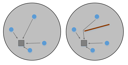
Without a barrier, the distance between a feature and a cell is the shortest one possible, that being a straight line between two points. With an open barrier, usually represented by a polyline, the path between a feature and a cell is influenced by the barrier. In this case, the distance between the feature and the cell is extended due to a detour around the barrier, as shown in the illustration below. As a result, the influence of the feature is reduced while estimating the density at the cell. The path around the barrier is created by connecting a series of straight lines to go around the barrier from the input point feature to the cell. It is still the shortest distance around the barrier but longer than the distance would be without the barrier. With a closed barrier, usually represented by a polygon completely encompassing a few features, the density calculation at a cell on one side of the barrier completely excludes the features on the other side of the barrier.

The kernel density operation with a barrier can provide the more realistic and accurate results in some situations compared to the kernel density without a barrier operation. For example, when exploring the density of the distribution of an amphibian species, the presence of a cliff or road may affect their movement. The cliff or road can be used as a barrier to get a better density estimation. Similarly, the result of a density analysis of the crime rate in a city may vary if a river that passes through the city is considered as a barrier.
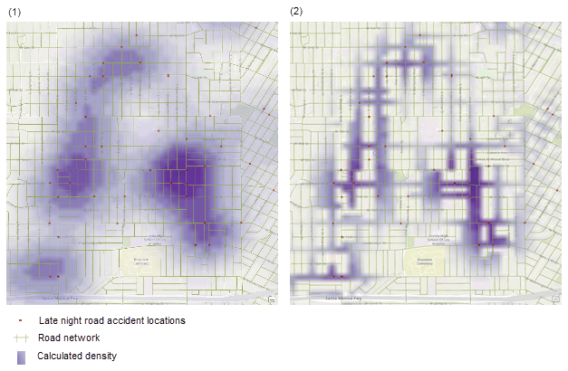
The illustration below shows the kernel density output of late-night traffic accidents in Los Angeles (data available from the Los Angeles County GIS Data Portal). The density estimation without a barrier is on the left (1) and with a barrier on both sides of the roads is on the right (2). The tool provides a much better estimation of density using the barrier, where the distance is measured along with the road network, than using the shortest distance between the accident locations.

References
Silverman, B. W. Density Estimation for Statistics and Data Analysis. New York: Chapman and Hall, 1986.